
From 2 geotiffs to a trained U-Net: 2D, 3D, and 4D imagery example. Part 1: Data
In this blog post, we present an end-to-end image segmetation workflow, using a small dataset, consisting of both imagery and digital elevation model (DEM). We are exploring a few goals:
- Can we use high-resolution RGB imagery with a U-Net model to segment sand dune types and forms
- Can we do so using a small dataset, using data augmentation?
- What creates the best prediction; RGB imagery alone? 2D elevation alone? Or the 4D combination of RGB and elevation?
This is a long workflow, so this blog post is split into two: data, then models. This post, 'Data', covers the following workflows:
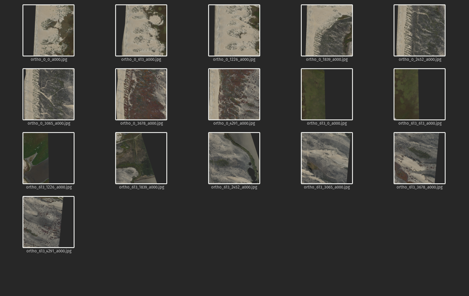
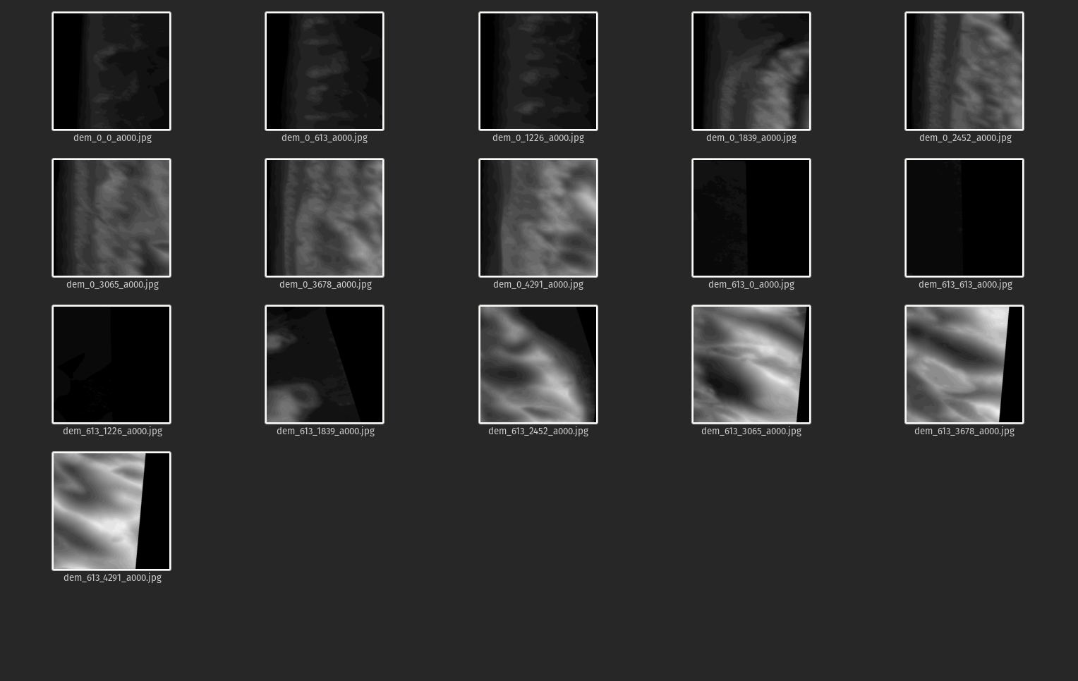
- Split large geoTIFF orthomosaics and DEMs into smaller tiles, using python and GDAL, for labelling and segmentation. This will create 9-bit RGB imagery and coincident 8-bit elevation data. Elevation can be negative, and is usually measured on a continuous scale, but we convert elevation values to positive relative discrete values. This relative elevation raster might be combined with the 3D imagery to create 4D raster stacks
- Convert imagery to jpeg format
- Use
dash_doodlerto semi-supervised image segmentation into 6 classes that relate to dune types and cover, and adjacent land cover. - The dataset is small - only 16 images, each only 613x613 pixels. Ordinarily for a deep learning project you would need MUCH more data. So, for this example we will use data augmentation to expand the dataset. In your adaptations of this workflow, you shouldn't rely so much on image augmentation and have more labelled examples. We use augmentation to create 64 new examples, each 608x608 pixels, which is the closest size to 613x613 pixels that will work with the U-Net model
- TFRecords are created from the 3D (RGB) imagery and the 2D (greyscale) labels
- TFRecords are created by combining 2D DEMs with 3D RGB imagery, with 2D (greyscale) labels
Dataset
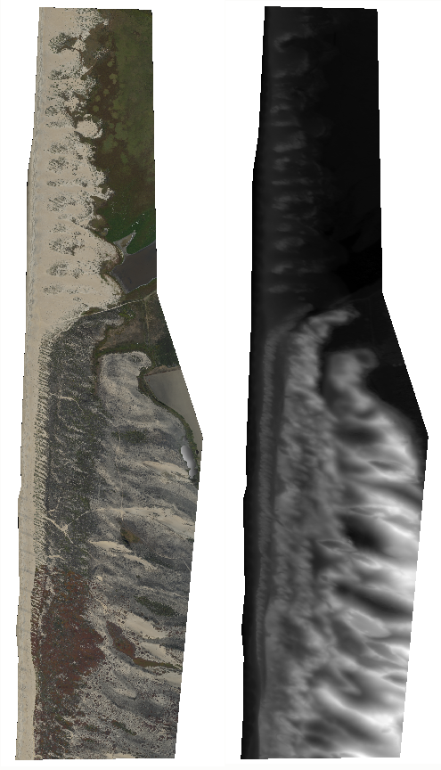
The dataset consists of a 50-cm orthomosaic and a 50-cm digital elevation model (DEM) of sand dunes in central Monterey Bay. These data were collected and processed by Jon Warrick and Andy Ritchie at the U.S Geological Survey Pacific Coastal & Marine Science Center, Santa Cruz, using Structure-from-Motion photogrammetry.
The GeoTiFF image (below, left) show incipient dunes (Northern, at the river mouth), established dunes without iceplant (Central), established dunes with iceplant (Southern). The iceplant is a non-native and has been weeded from the central portion by non-profits. You can see the iceplant in the southern section by the 'red' patches. There is a distinct difference in elevation in the incipient dunes and the established dunes (below, right).
Prepare dataset for ML labeling/training using python/GDAL
Load the libraries we need. We'll be using mostly system calls (from os.system) to GDAL libraries installed, such that the commands gdal_translate and gdal_calc.py are accessible. GDAL is cross-platform (install instructions)
import os
from glob import glob
Create RGB and DEM tiles
Define some inputs; the size of the tiles we would like to create, the files we'd like to tile, and their heights and widths
tilesize = 613

bigfiles = ['MontBay_Dunes_Ortho_50cm.tif', 'MontBay_Dunes_DEM_50cm.tif']
widths = [1226, 1226]
heights = [4930, 4930]
Create tiled geotiffs by calling gdal_translate as a system command, within a nested for-loop that first cycles through files, then position on a grid in x, then position on a grid in y, just applying the window (srcwin) flag
for k in range(len(bigfiles)):

    for i in range(0, widths[k], tilesize):
        for j in range(0, heights[k], tilesize):
            if 'Ortho' in bigfiles[k]:
                gdaltranString = "gdal_translate -of GTIFF -srcwin "+str(i)+", "+str(j)+", "+str(tilesize)+", " \
                +str(tilesize)+" "+bigfiles[k]+" ortho_"+str(i)+"_"+str(j)+".tif"
            else:
                gdaltranString = "gdal_translate -of GTIFF -srcwin "+str(i)+", "+str(j)+", "+str(tilesize)+", " \
                +str(tilesize)+" "+bigfiles[k]+" dem_"+str(i)+"_"+str(j)+".tif"
            os.system(gdaltranString)
These images are at the edge of the raster and are thus smaller than the rest. We'll delete them
os.system('rm dem*0_4904.tif')
os.system('rm ortho*0_4904.tif')
We need to add a scalar to every value in each DEM tile, to avoid negative numbers (negative elevation umbers occur in coastal data due to datum specifications). In this example the absolute elevation values are not important, only relative ones, because eventually the DEM will be discretized as an 8-bit raster with values ranging from 0 to 255. To ensure all negative numbers are not encoded 0, 40m is sufficient in this case.
voffset = 40 #vertical offset to avoid negative numbers

files = glob('dem*.tif')

for file in files:
    gdalstring = 'gdal_calc.py -A '+file+' --outfile='+file.replace('.tif', '_a0.tif')+'  --calc="(A+'+str(voffset)+')" --NoDataValue=0'
    os.system(gdalstring)
Next we'll ensure no remaining negative numbers (setting them to zero) and convert to 16-bit. In this case there are no negative numbers left, but this would be a generic way to enforce non-negativity
files = glob('dem*_a0.tif')

for file in files:
    gdalstring = 'gdal_calc.py -A '+file+' --outfile='+file.replace('_a0.tif', '_a00.tif')+'  --calc="A*(A>0)" --NoDataValue=0 --type=Int16'
    os.system(gdalstring)
The full range of elevation in the data set is 7 to 36 m. The next command will simultaneously convert the image to BYTE or 8-bit unsigned integer, which is the format we need going forward, and scale to the full range (0 to 255). And, it will convert from tiff to jpg format
files = glob('dem*_a00.tif')

for file in files:
    gdalstring = 'gdal_translate -of GTIFF -ot BYTE -scale 7 36 0 255 '+file+' '+file.replace('_a00.tif', '_a000.jpg')
    os.system(gdalstring)
Remove those intermediate files; we no longer need them
os.system('rm dem*a0.tif')
os.system('rm dem*a00.tif')
Convert each RGB image from tiff to jpg format. Actually these files won't be in jpeg encoding yet, only have the extension and bit-depth. We will correct the encoding later
files = glob('ortho*.tif')

for file in files:
    gdalstring = 'gdal_translate -of GTIFF -ot BYTE '+file+' '+file.replace('.tif', '_a000.jpg')
    os.system(gdalstring)
Then run the following bash command to enforce jpeg encoding for all the images, optionally writing new versions by profided a suffix e.g _c in front of the file extension (.jpg), such as here
for file in *.jpg; do convert $file $"${file%.jpg}_c.jpg"; done
Labeling images
We'll use the new protoype "dash doodler" tool that you can find here for rapidly annotating these 16 images. I could label the RGB imagery in doodler, but it isn't designed to accept more than 3-band imagery, and that format wouldn't be helpful (we'll see later on that RGB+DEM imagery just looks like the RGB image with the high parts whited out - not helpful, generally)
These are the 6 classes I'm interested in, written to classes.txt :
water
marsh
beach
incipient_foredune
established_dune
iceplant
Here is a video of me annotating all 16 images (actually this is a previous version where I labeled 8 classes - but you get the idea):
Doodler creates RGB and greyscale label images. RGB images are easier to see and evaluate, and they can be used to create TFRecords and segmentation workflows, like we saw in the OBX data example, but ultimately you have to decode the RGB image and that isn't necessarily easy to do. In fact that becomes hard to do when you have many classes and encode your labels as jpegs. The former because you have to use colors that tend to be increasingly similar the more classes you have, and compression and chroma subsampling used in jpeg creation isn't ideal at preserving those color values, so it becomes difficult to decode the labels. Jpeg compression isn't generally a problem for simple greyscale integer label images. That is why doodler creates greyscale images, and greyscale label imagery is what we will use going forward.
Image augmentation
We'll create a few more examples to create enough data for demonstration purposes. Ordinarily you would try to label much more data
Define image dimensions. The images are actually 613 x 613 pixels, but that won't fit within the U-Net framework without modification, so we'll resize to the nearest dimension that will, which is 608 x 608 pixels. Within the mlmondays conda environment,
from imports import *
NY = 608
NX = 608
Define two ImageDataGenerator instances with the same arguments, one for images and the other for labels (masks)
data_gen_args = dict(featurewise_center=False,
                     featurewise_std_normalization=False,
                     rotation_range=2,
                     width_shift_range=0.1,
                     height_shift_range=0.1,
                     zoom_range=0.1)
image_datagen = tf.keras.preprocessing.image.ImageDataGenerator(**data_gen_args)
dem_datagen = tf.keras.preprocessing.image.ImageDataGenerator(**data_gen_args)
mask_datagen = tf.keras.preprocessing.image.ImageDataGenerator(**data_gen_args)
Put your images somewhere and define the labels
imdir = 'data/dunes/images'

dem_path = 'data/dunes/dems'

lab_path = 'data/dunes/labels'
Note that you'll have to actually place your images inside another folder inside these respective directories, and it doesn't matter what that folder is called. The reason is that ImageDataGenerator expects imagery to be in class folders, even though in this case we are not using that functionality
Next, you'll need a function to write your images to file. We'll also use a median filter with a disk kernel (you'll need to install scikit-image to use these commands: conda install scikit-image)
from imageio import imwrite
from skimage.filters.rank import median
from skimage.morphology import disk
You likely can't read all your images into memory if you did augmentation on a real-sized dataset (i.e. bigger), so you'll likely have to do this in batches. Therefore we present the batched workflow.
The following loop will grab a new random batch of images, apply the augmentation generator to the images to create alternate versions, then writes those alternate versions of images and labels to disk. We use class_mode=None because the images don't belong to any particular class. The list L is for enumerating all the unique values of each label image, to check that no integers outside the class range are present.
L = []
i=1
for k in range(4): #create 4 more sets ....

    #set a different seed each time to get a new batch of ten
    seed = int(np.random.randint(0,100,size=1))
    img_generator = image_datagen.flow_from_directory(
            imdir,
            target_size=(NX, NY),
            batch_size=16, ## .... of 16 images ...
            class_mode=None, seed=seed, shuffle=True)

    dem_generator = image_datagen.flow_from_directory(
            dem_path,
            target_size=(NX, NY),
            batch_size=16, ## .... of 16 images ...
            class_mode=None, seed=seed, shuffle=True)

    #the seed must be the same as for the training set to get the same images
    mask_generator = mask_datagen.flow_from_directory(
            lab_path,
            target_size=(NX, NY),
            batch_size=16,  ## .... and of 16 labels
            class_mode=None, seed=seed, shuffle=True)

    #The following merges the 3 generators (and their flows) together:
    train_generator = (pair for pair in zip(img_generator, dem_generator, mask_generator))

    #grab a batch of images, dems, and label images
    x, y, z = next(train_generator)

    # write them to file and increment the counter
    for im,dem,lab in zip(x,y,z):
        imwrite(imdir+os.sep+'augimage_000'+str(i)+'.jpg', im)
        imwrite(dem_path+os.sep+'augdem_000'+str(i)+'.jpg', dem)

        lab = median(lab[:,:,0]/255.0, disk(3)).astype(np.uint8)
        lab[im[:,:,0]==0]=0
        L.append(np.unique(lab.flatten()))
        imwrite(lab_path+os.sep+'auglabel_000'+str(i)+'_label.jpg',(lab).astype(np.uint8))
        i += 1
        print(lab.shape)

    #save memory
    del x, y, im, dem, lab
    #get a new batch
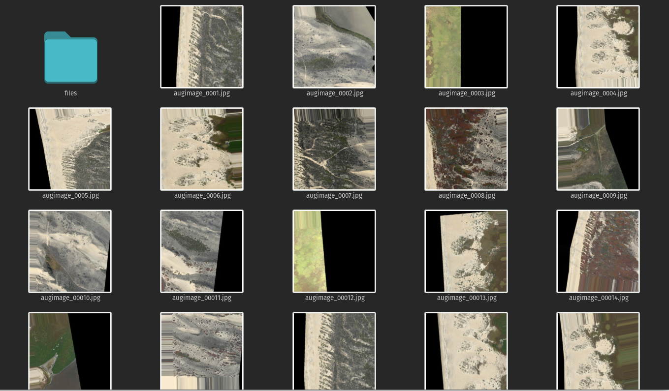
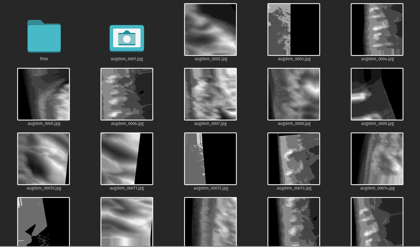
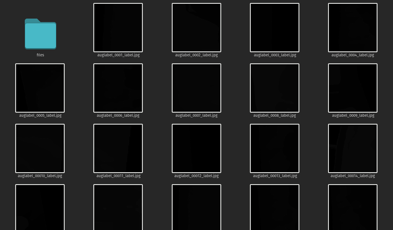
when this completes you should have 64 new images, dems and labels, that look something like this.
Images:
DEMs:
Labels:
What unique values do we have in our augmented imagery?
print(np.round(np.unique(np.hstack(L))))

[0 1 2 3 4 5 6 7 8]
Great. Zero for null, and our 1 through 6 classes
4D image creation
Now you have 64 images, dems and labels total. Next, we need to merge the images and dems together into 4-band images
But how do you make a 4-band image from a 3-band image and a 1-band image?
First, import libraries
from imageio import imread
import numpy as np
Read RGB image
im1 = imread('data/dunes/images/augimage_0001.jpg')
Read elevation and get just the first band
im2 = imread('data/dunes/dems/augdem_0001.jpg')[:,:,0]
Merge bands - creates a numpy array with 4 channels
merged = np.dstack((im1, im2))
Make this figure:
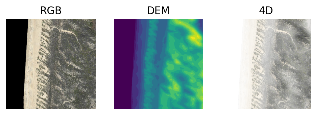
using this code:
import matplotlib.pyplot as plt
plt.subplot(131)
plt.imshow(im1); plt.axis('off'); plt.title('RGB')
plt.subplot(132)
plt.imshow(im2); plt.axis('off'); plt.title('DEM')
plt.subplot(133)
plt.imshow(merged); plt.axis('off'); plt.title('4D')
plt.savefig('4d.png', dpi=200, bbox_inches='tight'); plt.close('all')
TFRecord creation
Getting set up
With the mlmondays conda environment enabled, import some libraries:
from imports import *
from imageio import imwrite
Define our three paths:
imdir = '/media/marda/TWOTB/USGS/SOFTWARE/Projects/DL-CDI2020/3_ImageSeg/data/dunes/images'
demdir = '/media/marda/TWOTB/USGS/SOFTWARE/Projects/DL-CDI2020/3_ImageSeg/data/dunes/dems'
labdir = '/media/marda/TWOTB/USGS/SOFTWARE/Projects/DL-CDI2020/3_ImageSeg/data/dunes/labels'
And this path for the tfrecord files
tfrecord_dir = '/media/marda/TWOTB/USGS/SOFTWARE/Projects/DL-CDI2020/3_ImageSeg/data/dunes'
Define images per shard (12, so there will be SHARD=8 tfrecord files, since there are 48 images) and shard sizes
nb_images=len(tf.io.gfile.glob(imdir+os.sep+'*.jpg'))

ims_per_shard = 8

SHARDS = int(nb_images / ims_per_shard) + (1 if nb_images % ims_per_shard != 0 else 0)

shared_size = int(np.ceil(1.0 * nb_images / SHARDS))
List the images:
img_files = tf.io.gfile.glob(imdir+os.sep+'*.jpg')
Encode back to jpeg for efficient binary string storage
def recompress_seg_image(image, label):

    image = tf.cast(image, tf.uint8)
    image = tf.image.encode_jpeg(image, optimize_size=False, chroma_downsampling=False, quality=100)

    label = tf.cast(label, tf.uint8)
    label = tf.image.encode_jpeg(label, optimize_size=False, chroma_downsampling=False, quality=100)
    return image, label
3D workflow (R, G, B)
This function reads an image
def read_seg_image_and_label_dunes(img_path):
    bits = tf.io.read_file(img_path)
    image = tf.image.decode_jpeg(bits)

    dem_path = tf.strings.regex_replace(img_path, "images", "dems")
    dem_path = tf.strings.regex_replace(dem_path, "augimage", "augdem")
    bits = tf.io.read_file(dem_path)
    dem = tf.image.decode_jpeg(bits)

    # have to use this tf.strings.regex_replace utility because img_path is a Tensor object
    lab_path = tf.strings.regex_replace(img_path, "images", "labels")
    lab_path = tf.strings.regex_replace(lab_path, "augimage", "auglabel")
    lab_path = tf.strings.regex_replace(lab_path, ".jpg", "_label.jpg")
    bits = tf.io.read_file(lab_path)
    label = tf.image.decode_jpeg(bits, channels=1)

    label = tf.cast(label, tf.uint8)

    ## merge dem and image
    if flag is '3d':
      merged = tf.stack([image[:,:,0], image[:,:,1], image[:,:,2]], axis=2)
    elif flag is '3db':
      merged = tf.stack([image[:,:,0], image[:,:,2], dem[:,:,0]], axis=2)
    else:
      merged = tf.stack([image[:,:,0], image[:,:,1], image[:,:,2], dem[:,:,0]], axis=2)

    merged = tf.cast(merged, tf.uint8)

    return merged, label
flag='3d'
dataset = tf.data.Dataset.list_files(imdir+os.sep+'*.jpg', seed=10000) # This also shuffles the images
dataset = dataset.map(read_seg_image_and_label_dunes)
dataset = dataset.map(recompress_seg_image, num_parallel_calls=AUTO)
dataset = dataset.batch(shared_size)
Now we can write our 3D dataset out to TFRecords:
for shard, (image, label) in enumerate(dataset):
  shard_size = image.numpy().shape[0]
  filename = tfrecord_dir+os.sep+"dunes3d-" + "{:02d}-{}.tfrec".format(shard, shard_size)

  with tf.io.TFRecordWriter(filename) as out_file:
    for i in range(shard_size):
      example = to_seg_tfrecord(image.numpy()[i],label.numpy()[i])
      out_file.write(example.SerializeToString())
    print("Wrote file {} containing {} records".format(filename, shard_size))
4D workflow (R, G, B, DEM)
JPEGs can be either 1 or 4 bands, not 4 bands. So, we use a png encoder this time, which means we'll have to use a png decoder when we read the data in later for model training
def recompress_seg_image4d(image, label):

    image = tf.cast(image, tf.uint8)
    image = tf.image.encode_png(image)

    label = tf.cast(label, tf.uint8)
    label = tf.image.encode_png(label)
    return image, label
flag='4d'
dataset = tf.data.Dataset.list_files(imdir+os.sep+'*.jpg', seed=10000) # This also shuffles the images
dataset = dataset.map(read_seg_image_and_label_dunes)
dataset = dataset.map(recompress_seg_image4d, num_parallel_calls=AUTO)
dataset = dataset.batch(shared_size)
Now we can write our 4D dataset out to TFRecords:
for shard, (image, label) in enumerate(dataset):
  shard_size = image.numpy().shape[0]
  filename = tfrecord_dir+os.sep+"dunes4d-" + "{:02d}-{}.tfrec".format(shard, shard_size)

  with tf.io.TFRecordWriter(filename) as out_file:
    for i in range(shard_size):
      example = to_seg_tfrecord(image.numpy()[i],label.numpy()[i])
      out_file.write(example.SerializeToString())
    print("Wrote file {} containing {} records".format(filename, shard_size))