From 2 geotiffs to a trained U-Net: 2D, 3D, and 4D imagery example. Part 2: Models
Segmentation Model
In the previous post we prepared two analysis ready datasets, the first consisting of RGB (or 3D) images and associated greyscale labels, and the second consisting of 4D (RGB + DEM) imagery and the same labels. Here I show how to use that imagery in three different workflows, first using RGB imagery, then DEM, then a combination of the two. We'll evaluate using a validation dataset, and some unseen (unaugmented) sample imagery to test the ability of the model to generalize. We see that the 4D data is slightly better than the 3D data, which is a lot better than the 2D data for this task. However, in each case the model didn't do well on the sample imagery so some troubleshooting is required. Likely, a lot more data is required; this workflow uses only 16 original image tiles; many more would be required for accurate results. However, this blog post does demonstrate that the mlmondays workflows can be adapted to different data sets, and more complicated data and classes.
RGB imagery
Model preparation
from imports import *
def get_batched_dataset(filenames):

    option_no_order = tf.data.Options()
    option_no_order.experimental_deterministic = True

    dataset = tf.data.Dataset.list_files(filenames)
    dataset = dataset.with_options(option_no_order)
    dataset = dataset.interleave(tf.data.TFRecordDataset, cycle_length=16, num_parallel_calls=AUTO)
    dataset = dataset.map(read_seg_tfrecord_dunes, num_parallel_calls=AUTO)

    dataset = dataset.cache() # This dataset fits in RAM
    dataset = dataset.repeat()
    dataset = dataset.shuffle(2048)
    dataset = dataset.batch(BATCH_SIZE, drop_remainder=True) # drop_remainder will be needed on TPU
    dataset = dataset.prefetch(AUTO) #

    return dataset

def get_training_dataset():
    return get_batched_dataset(training_filenames)

def get_validation_dataset():
    return get_batched_dataset(validation_filenames)
We need a function to seg each example record from the TFRecord shards. You'll see similar functions in mlmondays workflows for OBX and OysterNet dataset. We start by creating a dictionary to use to parse the two features (image and label pair) as binary strings. Then convert each to jpeg and scale to the range [0, 1]. If any number in the label is greater than 8, it is set to zero. Zero is being used as a NULL class for zero image pixels. Finally, the label image is converted into a one-hot stack, with 9 bands (one for each of the 8 classes and the null class).
@tf.autograph.experimental.do_not_convert
def read_seg_tfrecord_dunes(example):
    features = {
        "image": tf.io.FixedLenFeature([], tf.string),  # tf.string = bytestring (not text string)
        "label": tf.io.FixedLenFeature([], tf.string),   # shape [] means scalar
    }
    # decode the TFRecord
    example = tf.io.parse_single_example(example, features)

    image = tf.image.decode_jpeg(example['image'], channels=3)
    image = tf.cast(image, tf.float32)/ 255.0

    label = tf.image.decode_jpeg(example['label'], channels=1)
    label = tf.cast(label, tf.uint8)

    cond = tf.greater(label, tf.ones(tf.shape(label),dtype=tf.uint8)*6)#8)
    label = tf.where(cond, tf.ones(tf.shape(label),dtype=tf.uint8)*0, label)

    label = tf.one_hot(tf.cast(label, tf.uint8), 7) #9)
    label = tf.squeeze(label)

    return image, label
From now on the code look should look familiar, if you've run through the exercises as part of mlmondays week 3 image segmentation. We define a data path to the tfrecord files, a filepath for the model weights, a file path for the training history plot. Then specify a patience for the early stopping criterion, the number of images encoded in each shard, for specification of training and validation steps per model training epoch, the validation split, and batch size.
data_path= os.getcwd()+os.sep+"data/dunes"

filepath = os.getcwd()+os.sep+'results/dunes_8class_best_weights_model.h5'

hist_fig = os.getcwd()+os.sep+'results/dunes_8class_model.png'

patience = 20

ims_per_shard = 12

VALIDATION_SPLIT = 0.6

BATCH_SIZE = 4

filenames = sorted(tf.io.gfile.glob(data_path+os.sep+'dunes3d*.tfrec'))

nb_images = ims_per_shard * len(filenames)
print(nb_images)

split = int(len(filenames) * VALIDATION_SPLIT)

training_filenames = filenames[split:]
validation_filenames = filenames[:split]

validation_steps = int(nb_images // len(filenames) * len(validation_filenames)) // BATCH_SIZE
steps_per_epoch = int(nb_images // len(filenames) * len(training_filenames)) // BATCH_SIZE
train_ds = get_training_dataset()

L = []
for k in range(12):
  plt.figure(figsize=(16,16))
  for imgs,lbls in train_ds.take(1):
    #print(lbls)
    for count,(im,lab) in enumerate(zip(imgs, lbls)):
       plt.subplot(int(BATCH_SIZE/2),int(BATCH_SIZE/2),count+1)
       plt.imshow(im)
       plt.imshow(np.argmax(lab,-1), cmap=plt.cm.bwr, alpha=0.5)#, vmin=0, vmax=7)
       #plt.imshow(lab, cmap=plt.cm.bwr, alpha=0.5, vmin=0, vmax=9)
       plt.axis('off')
       L.append(np.unique(np.argmax(lab,-1)))

  plt.show()
What unique values do we have in our augmented imagery?
print(np.round(np.unique(np.hstack(L))))

[0 1 2 3 4 5 6]
val_ds = get_validation_dataset()
Model training
Define the number of classes (9, including the null class) and target size (the encoded image's size), then create a model. Compile it, define callbacks.
nclasses=7 #9
TARGET_SIZE = 608
model = res_unet((TARGET_SIZE, TARGET_SIZE, 3), BATCH_SIZE, 'multiclass', nclasses)
# model.compile(optimizer = 'adam', loss = tf.keras.losses.CategoricalHinge(), metrics = [mean_iou])
model.compile(optimizer = 'adam', loss = 'categorical_crossentropy', metrics = [mean_iou])

earlystop = EarlyStopping(monitor="val_loss",
                              mode="min", patience=patience)

model_checkpoint = ModelCheckpoint(filepath, monitor='val_loss',
                                verbose=0, save_best_only=True, mode='min',
                                save_weights_only = True)

lr_callback = tf.keras.callbacks.LearningRateScheduler(lambda epoch: lrfn(epoch), verbose=True)

callbacks = [model_checkpoint, earlystop, lr_callback]
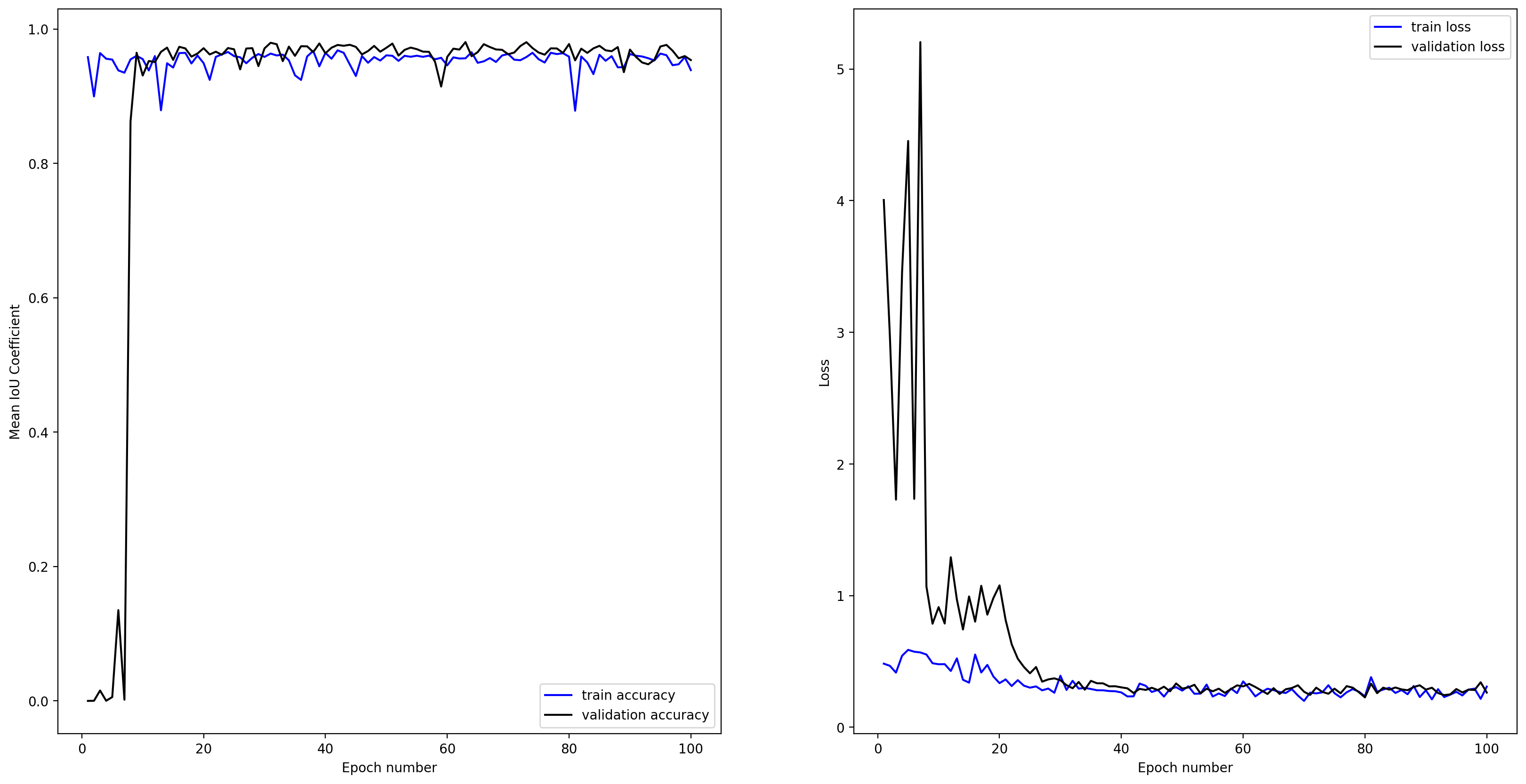
Fit the model, and make a plot of the model training history (loss and mean IOU).
#warmup
model.fit(train_ds, steps_per_epoch=steps_per_epoch, epochs=MAX_EPOCHS,
validation_data=val_ds, validation_steps=validation_steps,
callbacks=callbacks)
history = model.fit(train_ds, steps_per_epoch=steps_per_epoch, epochs=MAX_EPOCHS,
validation_data=val_ds, validation_steps=validation_steps,
callbacks=callbacks)
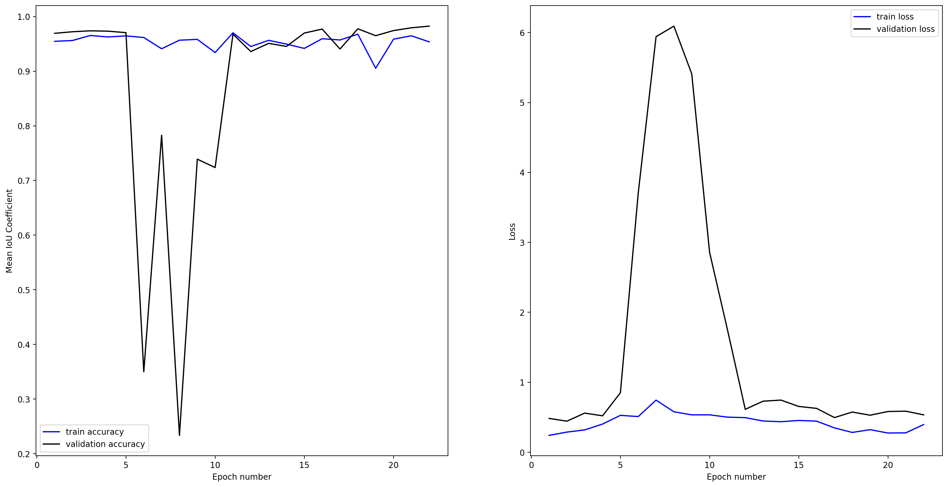
plot_seg_history_iou(history, hist_fig)
plt.close('all')
K.clear_session()
Model evaluation
Evaluate the model using the validation set. Print the average loss and IoU score.
scores = model.evaluate(val_ds, steps=validation_steps)

print('loss={loss:0.4f}, Mean IOU={iou:0.4f}'.format(loss=scores[0], iou=scores[1]))

loss=0.2917, Mean IOU=0.9542
sample_data_path = os.getcwd()+os.sep+'data/dunes/images/files'
test_samples_fig = os.getcwd()+os.sep+'dunes_sample_16class_est16samples.png'
sample_label_data_path = os.getcwd()+os.sep+'data/dunes/labels/files'

sample_filenames = sorted(tf.io.gfile.glob(sample_data_path+os.sep+'*.jpg'))
sample_label_filenames = sorted(tf.io.gfile.glob(sample_label_data_path+os.sep+'*.jpg'))
These are the same hex coolor codes as the plotly G10 colormap used to make the color label imagery, made into a custom matplotlib discrete colormap
from matplotlib.colors import ListedColormap
cmap = ListedColormap(["#000000",
      "#3366CC", "#DC3912",
      "#FF9900", "#109618",
      "#990099", "#0099C6"])#,
      # "#DD4477", "#66AA00"])
We're going to adopt a spatial filter again to remove high-frequency noise associated with jpeg compression and unpacking
from skimage.filters.rank import median
from skimage.morphology import disk
This is the same function as in the mlmondays repository, with the additional TARGET_SIZE argument
def seg_file2tensor(f, TARGET_SIZE):

    bits = tf.io.read_file(f)
    image = tf.image.decode_jpeg(bits)

    w = tf.shape(image)[0]
    h = tf.shape(image)[1]
    tw = TARGET_SIZE
    th = TARGET_SIZE
    resize_crit = (w * th) / (h * tw)
    image = tf.cond(resize_crit < 1,
                  lambda: tf.image.resize(image, [w*tw/w, h*tw/w]), # if true
                  lambda: tf.image.resize(image, [w*th/h, h*th/h])  # if false
                 )

    nw = tf.shape(image)[0]
    nh = tf.shape(image)[1]
    image = tf.image.crop_to_bounding_box(image, (nw - tw) // 2, (nh - th) // 2, tw, th)
    # image = tf.cast(image, tf.uint8) #/ 255.0

    return image
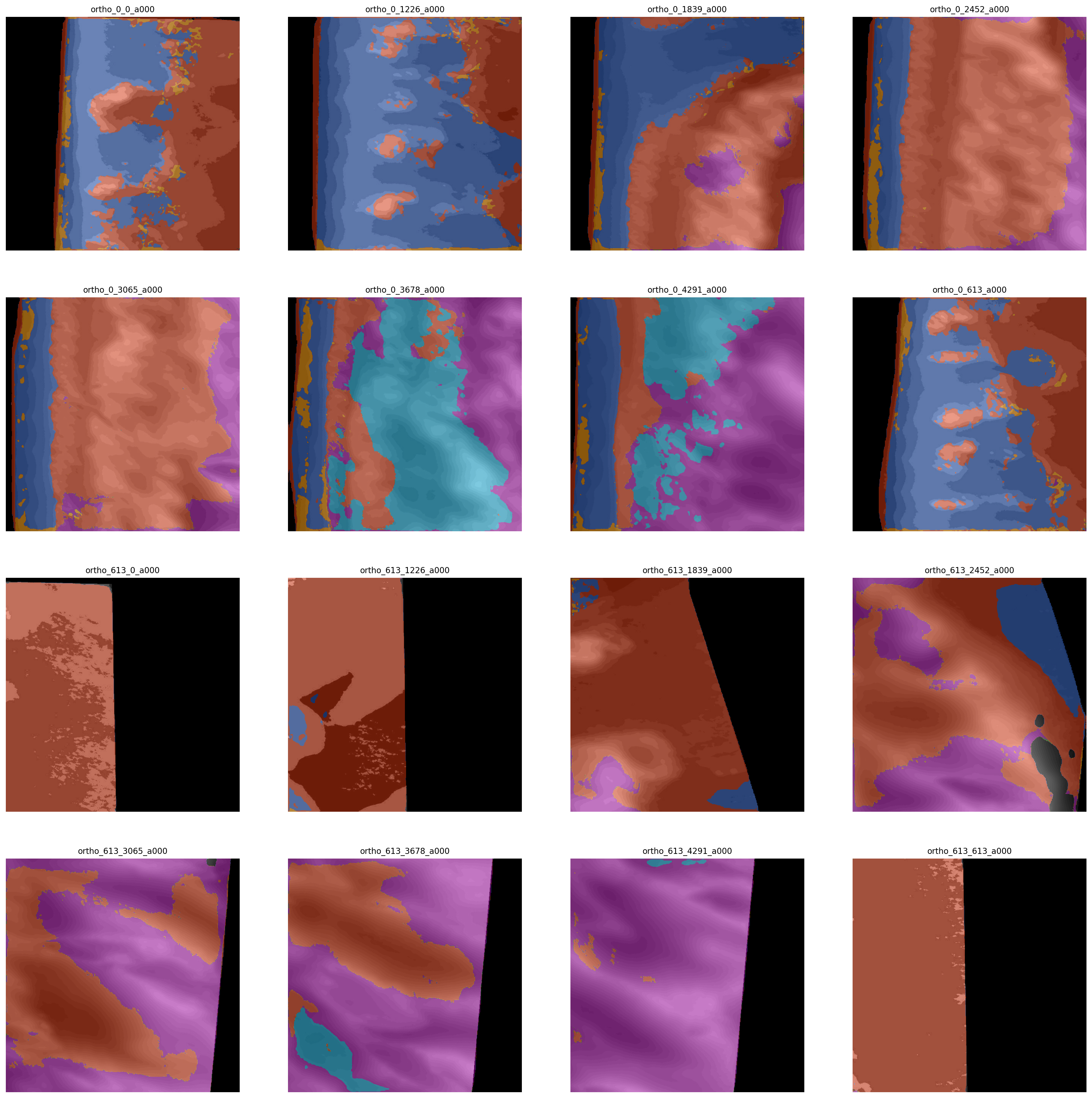
Cycle through each ground truth sample label image and create a list of those, L. Make a 4 x 4 subplot plot of the ground truth label images
L = []
plt.figure(figsize=(24,24))

for counter,(f,l) in enumerate(zip(sample_filenames, sample_label_filenames)):
    image = seg_file2tensor(f, TARGET_SIZE)
    label = seg_file2tensor(l, TARGET_SIZE)
    label = label.numpy().squeeze()

    label = median(label/255., disk(5)).astype(np.uint8)

    label[image[:,:,0]==0] = 0 #(0,0,0)

    plt.subplot(4,4,counter+1)
    name = sample_filenames[counter].split(os.sep)[-1].split('.jpg')[0]
    plt.title(name, fontsize=10)
    plt.imshow(image)

    plt.imshow(label, cmap=cmap, vmin=0, vmax=6) #8)

    plt.axis('off')
    L.append(label)

plt.savefig(test_samples_fig.replace('.png','_gt.png'),
            dpi=200, bbox_inches='tight')
plt.close('all')
These are the ground truth labels
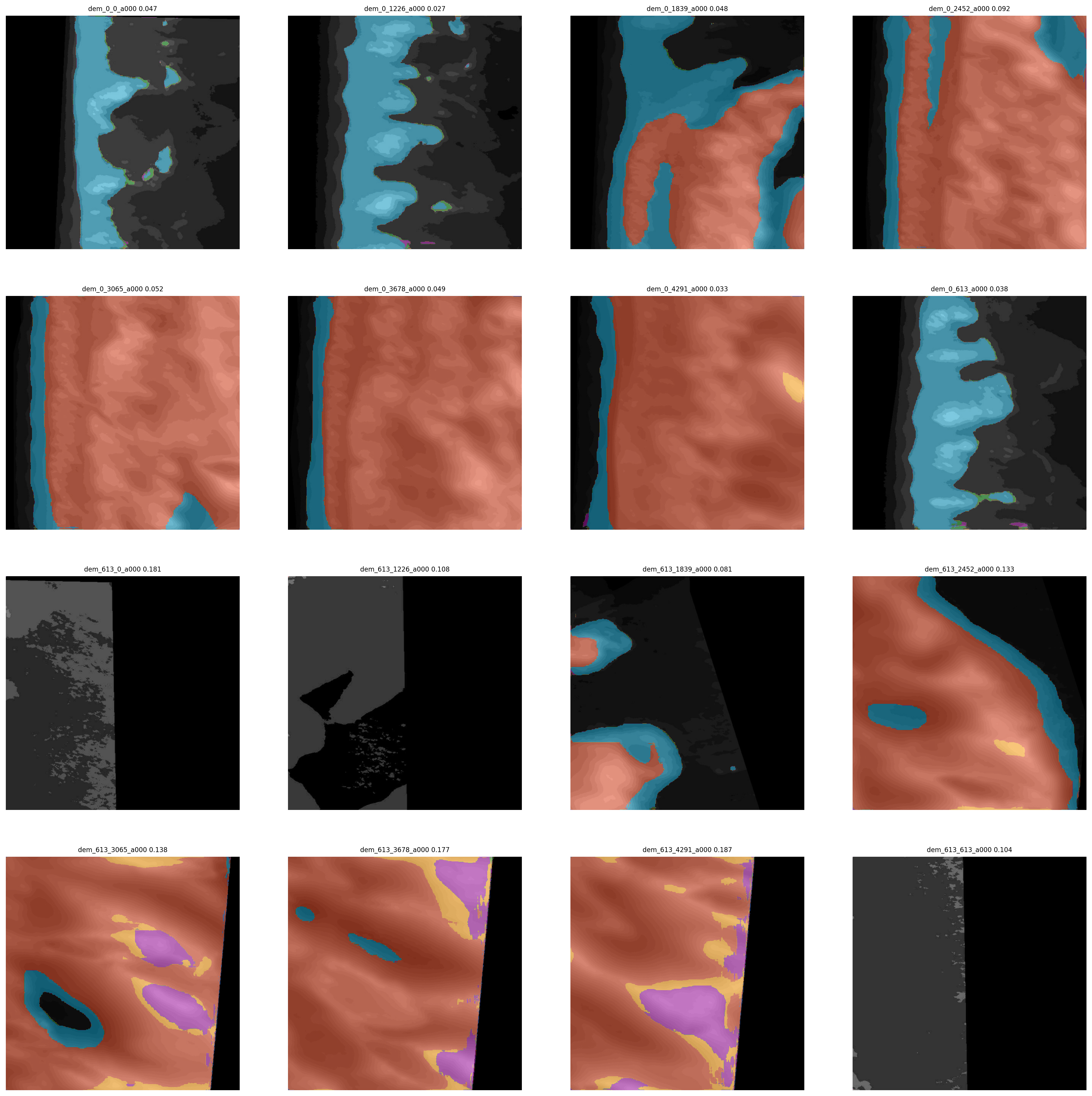
Cycle through each sample image and use the model to estimate the label image. Compare the one-hot encoded versions of the ground truth and prediction by computing a per-sample IoU score.
IOU = []
plt.figure(figsize=(24,24))

for counter,f in enumerate(sample_filenames):
    image = seg_file2tensor(f, TARGET_SIZE)/255
    est_label = model.predict(tf.expand_dims(image, 0) , batch_size=1).squeeze()

    est_labelp = tf.argmax(est_label, axis=-1)
    l = tf.one_hot(tf.cast(L[counter], tf.uint8), 7) #9)
    iou = mean_iou_np(np.expand_dims(l.numpy(),0), np.expand_dims(est_label,0))

    plt.subplot(4,4,counter+1)
    name = sample_filenames[counter].split(os.sep)[-1].split('.jpg')[0]
    plt.title(name+' '+str(iou)[:5], fontsize=12)
    plt.imshow(image)

    plt.imshow(est_labelp, alpha=0.5, cmap=cmap, vmin=0, vmax=6) #8)

    plt.axis('off')
    del est_labelp

    IOU.append(iou)

plt.savefig(test_samples_fig,
            dpi=200, bbox_inches='tight')
plt.close('all')
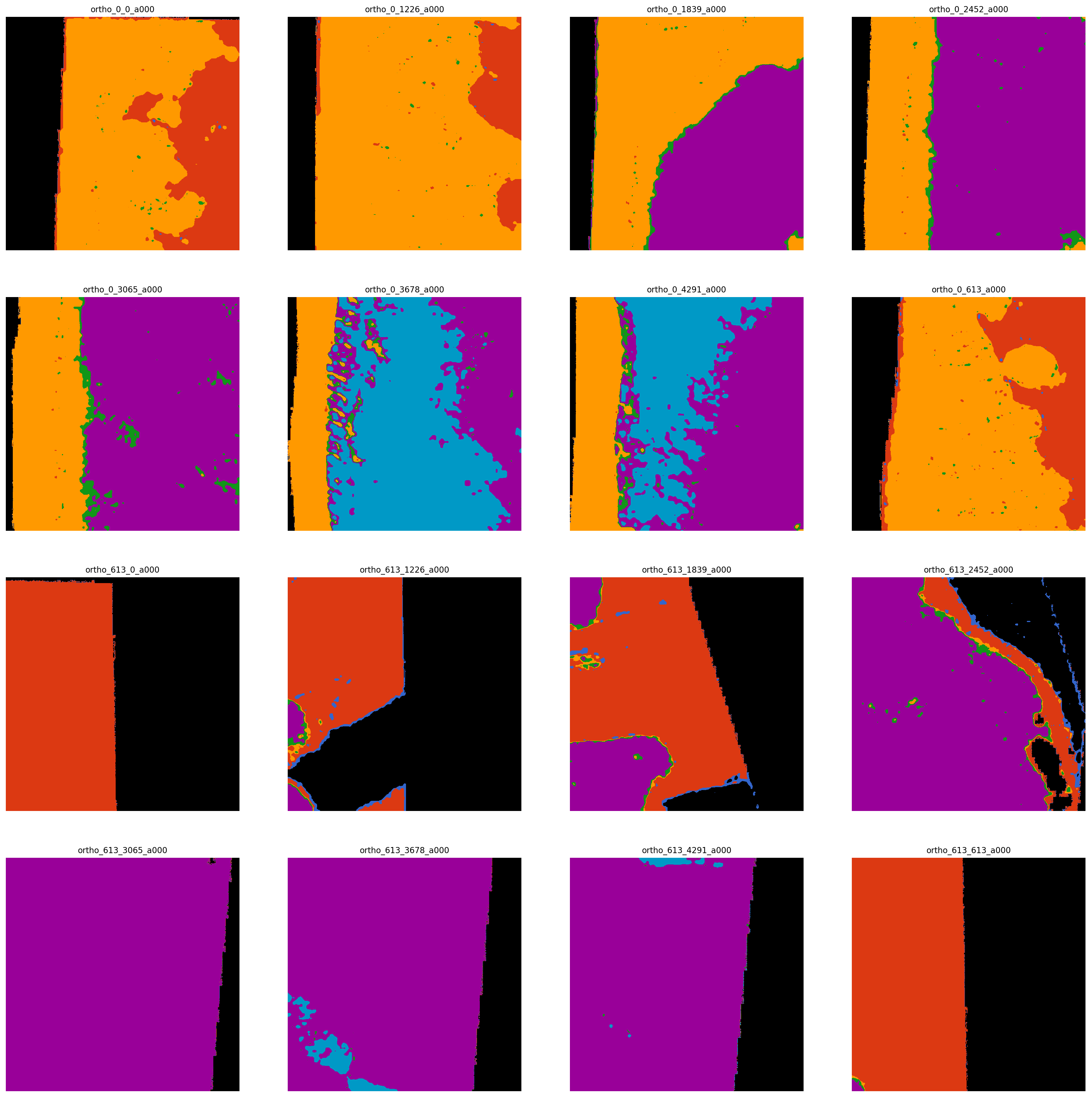
These are the predictions:
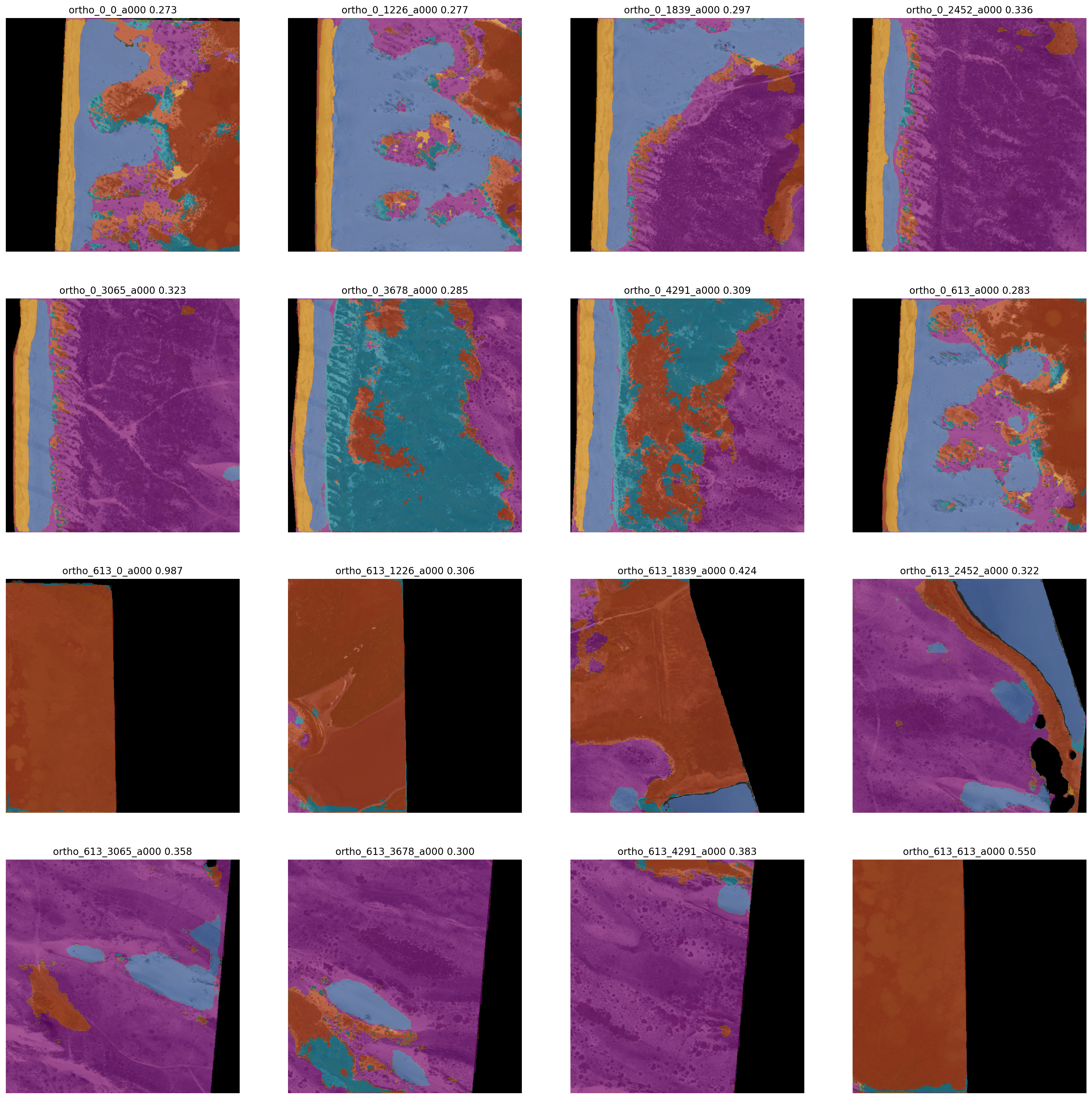
As you can see, the model does well at delineating the landscape but doesn't always get the class prediction correct. IoU scores are fairly low, 0.2, 0.4. The mean is only 0.3. This, I would confidently predict, is due to a lack of data. Big neural networks like this are designed for more independent examples.
Next we'll show the workflow and performance of a model trained to predict based on DEM alone
DEM imagery
Model preparation
For 2D imagery, we'll choose the DEM (last) channel in the 4D TFRecord stacks. SO we'll use the same function as before except returning image[:,:,-1] as the dem
@tf.autograph.experimental.do_not_convert
def read_seg_tfrecord_dunes(example):
    features = {
        "image": tf.io.FixedLenFeature([], tf.string),  # tf.string = bytestring (not text string)
        "label": tf.io.FixedLenFeature([], tf.string),   # shape [] means scalar
    }
    # decode the TFRecord
    example = tf.io.parse_single_example(example, features)

    image = tf.image.decode_png(example['image'], channels=1)
    image = tf.cast(image, tf.float32)/ 255.0

    label = tf.image.decode_jpeg(example['label'], channels=1)
    label = tf.cast(label, tf.uint8)

    cond = tf.greater(label, tf.ones(tf.shape(label),dtype=tf.uint8)*6) #8)
    label = tf.where(cond, tf.ones(tf.shape(label),dtype=tf.uint8)*0, label)

    label = tf.one_hot(tf.cast(label, tf.uint8), 7) #9)
    label = tf.squeeze(label)

    return image[:,:,-1], label
Redefine the variables for new files to contain the 2D results
data_path= os.getcwd()+os.sep+"data/dunes"

filepath = os.getcwd()+os.sep+'results/dunes2d_8class_best_weights_model.h5'

hist_fig = os.getcwd()+os.sep+'results/dunes2d_8class_model.png'

filenames = sorted(tf.io.gfile.glob(data_path+os.sep+'dunes4d*.tfrec'))

nb_images = ims_per_shard * len(filenames)
print(nb_images)

split = int(len(filenames) * VALIDATION_SPLIT)

training_filenames = filenames[split:]
validation_filenames = filenames[:split]

validation_steps = int(nb_images // len(filenames) * len(validation_filenames)) // BATCH_SIZE
steps_per_epoch = int(nb_images // len(filenames) * len(training_filenames)) // BATCH_SIZE
train_ds = get_training_dataset()
val_ds = get_validation_dataset()
Model training
Notice that the model is compiled with the input size (TARGET_SIZE, TARGET_SIZE, 1) rather than (TARGET_SIZE, TARGET_SIZE, 3) as before. Everything else is the same
model = res_unet((TARGET_SIZE, TARGET_SIZE, 1), BATCH_SIZE, 'multiclass', nclasses)
#model.compile(optimizer = 'adam', loss = tf.keras.losses.CategoricalHinge(), metrics = [mean_iou])
model.compile(optimizer = 'adam', loss = 'categorical_crossentropy', metrics = [mean_iou])

earlystop = EarlyStopping(monitor="val_loss",
                              mode="min", patience=patience)

model_checkpoint = ModelCheckpoint(filepath, monitor='val_loss',
                                verbose=0, save_best_only=True, mode='min',
                                save_weights_only = True)
We've decreased the data size, so I'm inclined to increase the learning rate a little. We'll set the parameters and redefine lrfn
start_lr = 1e-4
min_lr = start_lr
max_lr = 1e-3
rampup_epochs = 5
sustain_epochs = 0
exp_decay = .9

def lrfn(epoch):
    def lr(epoch, start_lr, min_lr, max_lr, rampup_epochs, sustain_epochs, exp_decay):
        if epoch < rampup_epochs:
            lr = (max_lr - start_lr)/rampup_epochs * epoch + start_lr
        elif epoch < rampup_epochs + sustain_epochs:
            lr = max_lr
        else:
            lr = (max_lr - min_lr) * exp_decay**(epoch-rampup_epochs-sustain_epochs) + min_lr
        return lr
    return lr(epoch, start_lr, min_lr, max_lr, rampup_epochs, sustain_epochs, exp_decay)


lr_callback = tf.keras.callbacks.LearningRateScheduler(lambda epoch: lrfn(epoch), verbose=True)
Fir the model and plot the training history as before
callbacks = [model_checkpoint, earlystop, lr_callback]

model.fit(train_ds, steps_per_epoch=steps_per_epoch, epochs=MAX_EPOCHS,
                      validation_data=val_ds, validation_steps=validation_steps,
                      callbacks=callbacks)


history = model.fit(train_ds, steps_per_epoch=steps_per_epoch, epochs=MAX_EPOCHS,
                      validation_data=val_ds, validation_steps=validation_steps,
                      callbacks=callbacks)

plot_seg_history_iou(history, hist_fig)

plt.close('all')
K.clear_session()
Model evaluation
Evaluate the model in the same way as for the 3D imagery case
scores = model.evaluate(val_ds, steps=validation_steps)

print('loss={loss:0.4f}, Mean IOU={iou:0.4f}'.format(loss=scores[0], iou=scores[1]))

loss=0.5537, Mean IOU=0.9835
sample_data_path = os.getcwd()+os.sep+'data/dunes/dems/files'

test_samples_fig = os.getcwd()+os.sep+'dunes2d_sample_16class_est16samples.png'

sample_filenames = sorted(tf.io.gfile.glob(sample_data_path+os.sep+'*.jpg'))

IOU = []
plt.figure(figsize=(24,24))

for counter,f in enumerate(sample_filenames):
    image = seg_file2tensor(f, TARGET_SIZE)/255
    est_label = model.predict(tf.expand_dims(image, 0) , batch_size=1).squeeze()

    est_labelp = tf.argmax(est_label, axis=-1)
    l = tf.one_hot(tf.cast(L[counter], tf.uint8), 7) #9)
    iou = mean_iou_np(np.expand_dims(l.numpy(),0), np.expand_dims(est_label,0))

    plt.subplot(4,4,counter+1)
    name = sample_filenames[counter].split(os.sep)[-1].split('.jpg')[0]
    plt.title(name+' '+str(iou)[:5], fontsize=8)
    plt.imshow(image, cmap=plt.cm.gray)

    plt.imshow(est_labelp, alpha=0.5, cmap=cmap, vmin=0, vmax=6) #8)

    plt.axis('off')
    del est_labelp

    IOU.append(iou)

plt.savefig(test_samples_fig,
            dpi=200, bbox_inches='tight')
plt.close('all')
Model not performing well at all on DEM data alone. A mean IoU score of around 0.1. This isn't particularly surprising; elevation is a poor descriptor of these classes alone, since marsh and beach are the same elevation, and bare and vegetated established dunes are also similar elevations.
RGB + DEM imagery
By combining RGB and DEM information together, the hope is that the model can exploit classes such as incipient foredune and iceplant that have distinct elevation zones, and make better distinctions between the other classes that differ in elevation characteristics.
Model preparation
@tf.autograph.experimental.do_not_convert
def read_seg_tfrecord_dunes(example):
    features = {
        "image": tf.io.FixedLenFeature([], tf.string),  # tf.string = bytestring (not text string)
        "label": tf.io.FixedLenFeature([], tf.string),   # shape [] means scalar
    }
    # decode the TFRecord
    example = tf.io.parse_single_example(example, features)

    image = tf.image.decode_png(example['image'], channels=4)
    image = tf.cast(image, tf.float32)/ 255.0

    label = tf.image.decode_jpeg(example['label'], channels=1)
    label = tf.cast(label, tf.uint8)

    cond = tf.greater(label, tf.ones(tf.shape(label),dtype=tf.uint8)*6) #8)
    label = tf.where(cond, tf.ones(tf.shape(label),dtype=tf.uint8)*0, label)

    label = tf.one_hot(tf.cast(label, tf.uint8), 7) #9)
    label = tf.squeeze(label)

    return image, label
data_path= os.getcwd()+os.sep+"data/dunes"

filepath = os.getcwd()+os.sep+'results/dunes4d_8class_best_weights_model.h5'

hist_fig = os.getcwd()+os.sep+'results/dunes4d_8class_model.png'

filenames = sorted(tf.io.gfile.glob(data_path+os.sep+'dunes4d*.tfrec'))

nb_images = ims_per_shard * len(filenames)
print(nb_images)

split = int(len(filenames) * VALIDATION_SPLIT)

training_filenames = filenames[split:]
validation_filenames = filenames[:split]

validation_steps = int(nb_images // len(filenames) * len(validation_filenames)) // BATCH_SIZE
steps_per_epoch = int(nb_images // len(filenames) * len(training_filenames)) // BATCH_SIZE

train_ds = get_training_dataset()

val_ds = get_validation_dataset()
Another thing you could play with is the kernel size used in the convolutional layers of the UNet. Previously that was set to 3 by default. Below I increase that to 5, in the hope a larger receptive field will mean greater elevation-image covariation scales to be captured.
def res_unet(sz, f, flag, nclasses=1):
    inputs = tf.keras.layers.Input(sz)

    ## downsample
    e1 = bottleneck_block(inputs, f, kernel_size=(5, 5)); f = int(f*2)
    e2 = res_block(e1, f, strides=2, kernel_size=(5, 5)); f = int(f*2)
    e3 = res_block(e2, f, strides=2, kernel_size=(5, 5)); f = int(f*2)
    e4 = res_block(e3, f, strides=2, kernel_size=(5, 5)); f = int(f*2)
    _ = res_block(e4, f, strides=2, kernel_size=(5, 5))

    ## bottleneck
    b0 = conv_block(_, f, strides=1)
    _ = conv_block(b0, f, strides=1)

    ## upsample
    _ = upsamp_concat_block(_, e4)
    _ = res_block(_, f, kernel_size=(5, 5)); f = int(f/2)

    _ = upsamp_concat_block(_, e3)
    _ = res_block(_, f, kernel_size=(5, 5)); f = int(f/2)

    _ = upsamp_concat_block(_, e2)
    _ = res_block(_, f, kernel_size=(5, 5)); f = int(f/2)

    _ = upsamp_concat_block(_, e1)
    _ = res_block(_, f, kernel_size=(5, 5))

    ## classify
    if flag is 'binary':
        outputs = tf.keras.layers.Conv2D(nclasses, (1, 1), padding="same", activation="sigmoid")(_)
    else:
        outputs = tf.keras.layers.Conv2D(nclasses, (1, 1), padding="same", activation="softmax")(_)

    #model creation
    model = tf.keras.models.Model(inputs=[inputs], outputs=[outputs])
    return model
Model training
Everything the same as before except the (TARGET_SIZE, TARGET_SIZE, 4) indicating a 4th input dimension
model = res_unet((TARGET_SIZE, TARGET_SIZE, 4), BATCH_SIZE, 'multiclass', nclasses)
# model.compile(optimizer = 'adam', loss = tf.keras.losses.CategoricalHinge(), metrics = [mean_iou])
model.compile(optimizer = 'adam', loss = 'categorical_crossentropy', metrics = [mean_iou])

earlystop = EarlyStopping(monitor="val_loss",
                              mode="min", patience=patience)

model_checkpoint = ModelCheckpoint(filepath, monitor='val_loss',
                                verbose=0, save_best_only=True, mode='min',
                                save_weights_only = True)
Increase learning rate (again, we're just simulating things you could change rather than necessarily be the optimal hyperparameters)
start_lr = 1e-6 #0.00001
min_lr = start_lr
max_lr = 1e-3
rampup_epochs = 5
sustain_epochs = 0
exp_decay = .9

def lrfn(epoch):
    def lr(epoch, start_lr, min_lr, max_lr, rampup_epochs, sustain_epochs, exp_decay):
        if epoch < rampup_epochs:
            lr = (max_lr - start_lr)/rampup_epochs * epoch + start_lr
        elif epoch < rampup_epochs + sustain_epochs:
            lr = max_lr
        else:
            lr = (max_lr - min_lr) * exp_decay**(epoch-rampup_epochs-sustain_epochs) + min_lr
        return lr
    return lr(epoch, start_lr, min_lr, max_lr, rampup_epochs, sustain_epochs, exp_decay)


lr_callback = tf.keras.callbacks.LearningRateScheduler(lambda epoch: lrfn(epoch), verbose=True)

callbacks = [model_checkpoint, earlystop, lr_callback]
Fit the model
#warm start
model.fit(train_ds, steps_per_epoch=steps_per_epoch, epochs=MAX_EPOCHS,
                      validation_data=val_ds, validation_steps=validation_steps,
                      callbacks=callbacks)

history = model.fit(train_ds, steps_per_epoch=steps_per_epoch, epochs=MAX_EPOCHS,
                      validation_data=val_ds, validation_steps=validation_steps,
                      callbacks=callbacks)

plot_seg_history_iou(history, hist_fig)

plt.close('all')
K.clear_session()
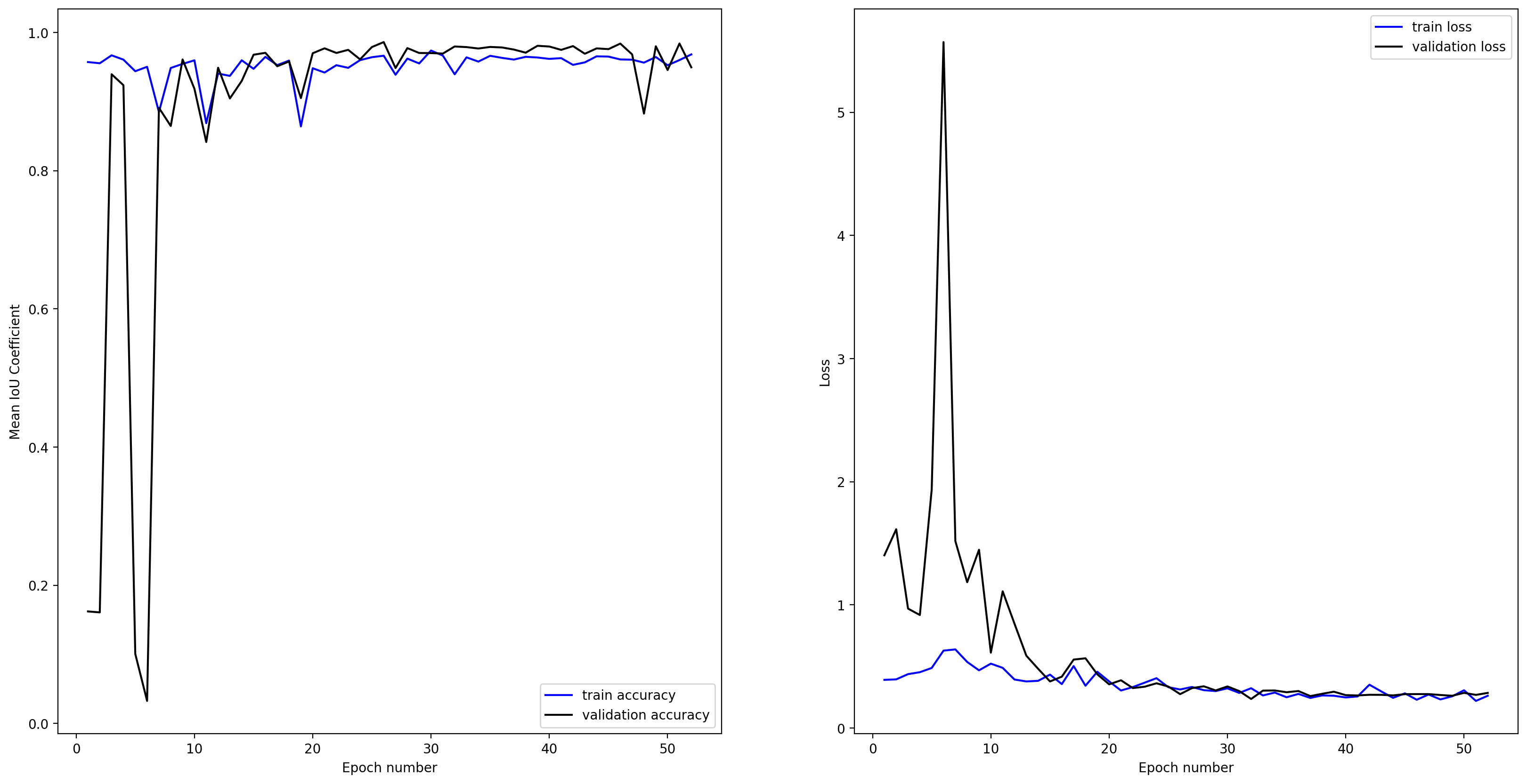
Model evaluation
Evaluate the same way as previously
scores = model.evaluate(val_ds, steps=validation_steps)

print('loss={loss:0.4f}, Mean IOU={iou:0.4f}'.format(loss=scores[0], iou=scores[1]))

loss=0.2936, Mean IOU=0.9748
Almost identical to the 3D example
sample_data_path = os.getcwd()+os.sep+'data/dunes/images/files'

test_samples_fig = os.getcwd()+os.sep+'dunes4d_sample_16class_est16samples.png'

sample_filenames = sorted(tf.io.gfile.glob(sample_data_path+os.sep+'*.jpg'))
IOU = []
plt.figure(figsize=(24,24))

for counter,f in enumerate(sample_filenames):
    image = seg_file2tensor(f, TARGET_SIZE)/255

    dem = seg_file2tensor(f.replace('images','dems').replace('ortho','dem'), TARGET_SIZE)/255

    merged = np.dstack((image.numpy(), dem.numpy()[:,:,0]))

    est_label = model.predict(tf.expand_dims(merged, 0) , batch_size=1).squeeze()

    l = tf.one_hot(tf.cast(L[counter], tf.uint8), 7) #9)
    iou = mean_iou_np(np.expand_dims(l.numpy(),0), np.expand_dims(est_label,0))

    est_label = tf.argmax(est_label, axis=-1)

    plt.subplot(4,4,counter+1)
    name = sample_filenames[counter].split(os.sep)[-1].split('.jpg')[0]
    plt.title(name, fontsize=10)
    plt.imshow(dem, cmap=plt.cm.gray)

    plt.imshow(est_label, alpha=0.5, cmap=cmap, vmin=0, vmax=6) #8)

    plt.axis('off')

    IOU.append(iou)

# plt.show()
plt.savefig(test_samples_fig,
            dpi=200, bbox_inches='tight')
plt.close('all')
Again, only an IOU of 0.32 - a marginal improvement over the 3D data. But overall I conclude that 1) you can use 2D, 3D, or 4D imagery with a U-Net and get a reasonable segmentation, however 2) I hypothesize that this workflow requires much more data. I achieved similar results with 8 classes.